functions for inspecting data

summary : describe files associated with a dataset

climaf.functions.summary(dat)

Summary provides the informations on a CliMAF dataset or ensemble of datsets It displays the path and filenames, and the dictionary of pairs keyword-values associated with the dataset.

>>> dat= ds(....)   # some dataset, with whatever variable
>>> summary(dat) #

ncdump : dump file header

• ncdump : show only the header information of a netCDF file

cshow : dump an object

climaf.driver.cshow(obj)

Provide the in-memory value of a CliMAF object. For a figure object, this will lead to display it ( launch computation if needed. )

functions to create images, and to display datasets and images

Warning

SEE ALSO the graphic operators and especially plot : map, cross-section and profile plot of one or two fields, and vectors plot over a map

ncview: display a dataset

• ncview : launch ncview on a dataset

iplot : Interactive version of cshow() for display in IPython Notebooks

climaf.functions.iplot(map)

implot : Interactive version of plot() for display in IPython Notebooks

climaf.functions.implot(field, **kwargs)

ts_plot : Shortcut for ensemble_ts_plot

climaf.functions.ts_plot(ts, **kwargs)

A python-user-friendly interface for the climaf operator ensemble_ts_plot : plot time series.

It takes the same arguments, but you can pass python lists instead of comma-separared strings.

It can take as input:

• a single CliMAF object dataset alone
• a dictionary with a name and a single CliMAF object
• a list of dictionaries or CliMAF objects
• a CliMAF ensemble

It is also able to take ‘title’ and ‘title_fontsize ‘as argument (will use the right_string resource for this)

See the documentation of ensemble_ts_plot : plot time series for the details on all possible options.

Examples

>>> ds= ....   # some dataset, with whatever variable
>>> ts_ds = space_avarege(ds) # Compute the space average
>>> p1 = ts_plot(ts_ds) # -- Simply provide the CliMAF object
>>> p2 = ts_plot({'my_dataset':ts_ds}) # -- Same as above but specify the name associated with the time series in the plot
>>> p3 = ts_plot([ts_ds1,ts_ds2,ts_ds3])
>>> p4 = ts_plot([ {'ts_ds1':ts_ds1}, {'ts_ds2':ts_ds2}, {'ts_ds3':ts_ds3} ]) # -- provide multiple time series in a given order with names
>>> p5 = ts_plot([ {'ts_ds1':ts_ds1}, {'ts_ds2':ts_ds2}, {'ts_ds3':ts_ds3} ], title='Three Time series', colors=['black','blue','red']) # -- Same as above with lines colors and title

>>> ens_ts = cens({'ts_ds1':ts_ds1, 'ts_ds2':ts_ds2, 'ts_ds3':ts_ds3}, order=['ts_ds1','ts_ds2','ts_ds3'])
>>> ens_ts.set_order(['ts_ds1','ts_ds2','ts_ds3'])
>>> p4bis = ts_plot(ens_ts) # -- Same result as p4 above but providing a CliMAF ensemble with specified order

plot_params : get plot parameters for a variable and a context

climaf.plot.plot_params.plot_params(variable, context, custom_plot_params=None)

Returns a dictionary of default plotting parameters (isolines, color palettes...) by variable and context, i.e. the full field (full_field), bias (bias), or model-model difference (model_model).

This type of dictionary is typically passed to plot with “**”.

plot_params first loads a set of default CliMAF plotting parameters for both ‘atmos’ and ‘ocean’.

Then, it updates with sets of parameters that are specific to the centers (for instance CNRM or IPSL).

Eventually, it can take a custom dictionary as an argument; it will use it to update the dictionary (i.e. override matching entries). Such a dictionnary would be build such as the example at ../climaf/plot/atmos_plot_params.py

Parameters:

• variable (string) – variable name; The name of the geophysical variable to plot
• context (string) – among ‘full_field’, ‘bias’, ‘model_model’; The kind of plot
• custom_plot_params – a user dictionnary that will override CliMAF default values

Returns : a python dictionary with plotting parameters to be used by plot()

Call example

>>> var = 'pr'
>>> climato_dat = time_average(ds(variable=var, project='CMIP5', ...))       # here, the annual mean climatology of a CMIP5 dataset for variable var
>>> climato_ref = time_average(ds(variable=var, project='ref_climatos',...)) # the annual mean climatology of a reference dataset for variable var

>>> bias = diff_regrid(climato_dat,climato_ref)         # We compute the bias map with diff_regrid()
>>> niceplot_params=**plot_params(var,'full_field')
>>> climato_plot = plot(climato_dat, nice_plot_params)
>>> bias_plot = plot(bias, **plot_params(var,'bias'))

>>> my_custom_params = {'pr':{'bias':{'colors':'-10 -5 -2 -0.5 -0.2 -0.1 0 0.1 0.2 0.5 1 2 5 10'}}}
>>> bias_plot_custom_params = plot(bias, **plot_params(var,'bias',custom_plot_params=my_custom_params)

>>> # How to import custom params stored in a my_custom_plot_param_file.py file in the working directory
>>> from my_custom_plot_param_file import dict_plot_params as my_custom_params
>>> bias_plot_custom_params = plot(bias, **plot_params(var,'bias',custom_plot_params=my_custom_params)

hovm_params : provide some SST/climate boxes for plotting Hovmoller diagrams

climaf.plot.plot_params.hovm_params(SSTbox_name)

Returns a dictionary with domain definition of SST/climate specified box for plotting Hovmoller diagrams

This type of dictionary is typically passed to ‘hovm’ operator with “**”.

Arg:

SSTbox_name (string) : SST/climate box name. The available boxes are: ‘NINO3-4’, ‘NINO1-2’, ‘NINO3’, ‘NINO4’, ‘GRL’, ‘NATL’, ‘SAT’ and ‘TPA’.

Returns : a python dictionary with domain parameters (‘latS’, ‘latN’, ‘lonW’, ‘lonE’) to be used by hovm()

Call example

>>> tas=ds(project='example', simulation='AMIPV6ALB2G', variable='tas', frequency='monthly', period='1980')
>>> # We plot a Hovmoller diagram (t,y) at longitude close to 10 for 'NINO1-2' domain
>>> hov_diag=hovm(tas, mean_axis='Point', xpoint=10., title='Temperature', **hovm_params('NINO1-2'))
>>> cfile(hov_diag)

cshow : display a figure using ‘display’

climaf.driver.cshow(obj)

Provide the in-memory value of a CliMAF object. For a figure object, this will lead to display it ( launch computation if needed. )

functions for assembling figures in pages

For choosing between next two fuctnions, see the Note on figure pages

cpage : create an array of figures (output: ‘png’ or ‘pdf’ figure)

class climaf.classes.cpage(fig_lines=None, widths=None, heights=None, fig_trim=True, page_trim=True, format='png', orientation=None, page_width=1000.0, page_height=1500.0, title='', x=0, y=26, ybox=50, pt=24, font='Times-New-Roman', gravity='North', background='white')

Builds a CliMAF cpage object, which represents an array of figures (output: ‘png’ or ‘pdf’ figure)

Parameters:

• fig_lines (a list of lists of figure objects or an ensemble of figure objects) – each sublist of ‘fig_lines’ represents a line of figures
• widths (list, optional) –

  the list of figure widths, i.e. the width of each column. By default, if fig_lines is:

  • a list of lists: spacing is even
  • an ensemble: one column is used

• heights (list, optional) – the list of figure heights, i.e. the height of each line. By default spacing is even
• fig_trim (logical, optional) – to turn on/off triming for all figures. It removes all the surrounding extra space of figures in the page, either True (default) or False
• page_trim (logical, optional) – to turn on/off triming for the page. It removes all the surrounding extra space of the page, either True (default) or False
• format (str, optional) – graphic output format, either ‘png’ (default) or ‘pdf’(not recommended)
• page_width (float, optional) – width resolution of resultant image; CLiMAF default: 1000.
• page_height (float, optional) – height resolution of resultant image; CLiMAF default: 1500.
• orientation (str,optional) – if set, it supersedes page_width and page_height with values 1000*1500 (for portrait) or 1500*1000 (for landscape)
• title (str, optional) – append a label below or above (depending optional argument ‘gravity’) figures in the page.

If title is activated:

• x, y (int, optional): annotate the page with text. x is the offset towards the right from the upper left corner of the page, while y is the offset upward or the bottom according to the optional argument ‘gravity’ (i.e. ‘South’ or ‘North’ respectively); CLiMAF default: x=0, y=26. For more details, see: http://www.imagemagick.org/script/command-line-options.php?#annotate ; where x and y correspond respectively to tx and ty in -annotate {+-}tx{+-}ty text
• ybox (int, optional): width of the assigned box for title; CLiMAF default: 50. For more details, see: http://www.imagemagick.org/script/command-line-options.php?#splice
• pt (int, optional): font size of the title; CLiMAF default: 24
• font (str, optional): set the font to use when creating title; CLiMAF default: ‘Times-New-Roman’. To print a complete list of fonts, use: ‘convert -list font’
• gravity (str, optional): the choosen direction specifies where to position title; CLiMAF default: ‘North’. For more details, see: http://www.imagemagick.org/script/command-line-options.php?#gravity
• background (str, optional): background color of the assigned box for title; default: ‘white’. To print a complete list of color names, use: ‘convert -list color’

Example

Using no default value, to create a page with 2 columns and 3 lines:

>>> tas_ds=ds(project='example',simulation='AMIPV6ALB2G', variable='tas', period='1980-1981')
>>> tas_avg=time_average(tas_ds)
>>> fig=plot(tas_avg,title='title')
>>> my_page=cpage([[None, fig],[fig, fig],[fig,fig]], widths=[0.2,0.8],
... heights=[0.33,0.33,0.33], fig_trim=False, page_trim=False,
... format='pdf', title='Page title', x=10, y=20, ybox=45,
... pt=20, font='Utopia', gravity='South', background='grey90',
... page_width=1600., page_height=2400.)

cpage_pdf : create an array of figures (output: ‘pdf’ figure)

class climaf.classes.cpage_pdf(fig_lines=None, widths=None, heights=None, orientation=None, page_width=1000.0, page_height=1500.0, scale=1.0, openright=False, title='', x=0, y=2, titlebox=False, pt='Huge', font='\familydefault', background='white')

Builds a CliMAF cpage_pdf object, which represents an array of figures (output: ‘pdf’ figure). Figures are automatically centered in the page using ‘pdfjam’ tool; see http://www2.warwick.ac.uk/fac/sci/statistics/staff/academic-research/firth/software/pdfjam

Parameters:

• fig_lines (a list of lists of figure objects or an ensemble of figure objects) – each sublist of ‘fig_lines’ represents a line of figures
• widths (list, optional) –

  the list of figure widths, i.e. the width of each column. By default, if fig_lines is:

  • a list of lists: spacing is even
  • an ensemble: one column is used

• heights (list, optional) – the list of figure heights, i.e. the height of each line. By default spacing is even
• page_width (float, optional) – width resolution of resultant image; CLiMAF default: 1000.
• page_height (float, optional) – height resolution of resultant image; CLiMAF default: 1500.
• orientation (str,optional) – if set, it supersedes page_width and page_height with values 1000*1500 (for portrait) or 1500*1000 (for landscape)
• scale (float, optional) – to scale all input pages; default:1.
• openright (logical, optional) – this option puts an empty figure before the first figure; default: False. For more details, see: http://ftp.oleane.net/pub/CTAN/macros/latex/contrib/pdfpages/pdfpages.pdf
• title (str, optional) – append a label in the page.

If title is activated, it is by default horizontally centered:

• x (int, optional): title horizontal shift (in cm).
• y (int, optional): vertical shift from the top of the page (in cm); only positive (down) values have an effect, default=2 cm
• titlebox (logical, optional): set it to True to frame the text in a box, frame color is ‘black’
• pt (str, optional): title font size; CLiMAF default: ‘Huge’ (corresponding to 24 pt). You can set or not a backslash before this argument.
• font (str, optional): font abbreviation among available LaTex fonts; default: ‘\\familydefault’.
• background (str, optional): frame fill background color; among LaTex ‘fcolorbox’ colors; default: ‘white’.

Left and right margins are set to 2cm.

Example

Using no default value, to create a PDF page with 2 columns and 3 lines:

>>> tas_ds=ds(project='example',simulation='AMIPV6ALB2G', variable='tas', period='1980-1981')
>>> tas_avg=time_average(tas_ds)
>>> fig=plot(tas_avg,title='title',format='pdf')
>>> crop_fig=cpdfcrop(fig)
>>> my_pdfpage=cpage_pdf([[crop_fig,crop_fig],[crop_fig, crop_fig],[crop_fig,crop_fig]],
... widths=[0.2,0.8], heights=[0.33,0.33,0.33], page_width=800., page_height=1200.,
... scale=0.95, openright=True, title='Page title', x=-5, y=10, titlebox=True,
... pt='huge', font='ptm', background='yellow') # Font name is 'Times'

html : package for creating an html index, with tables of links to figures

CliMAF module html defines functions for building some html index giving acces to figure files, through links bearing a label or through thumbnails. It eases iterating over lines and columns in tables.

See a code example in index_html.py or a screen dump for a similar code here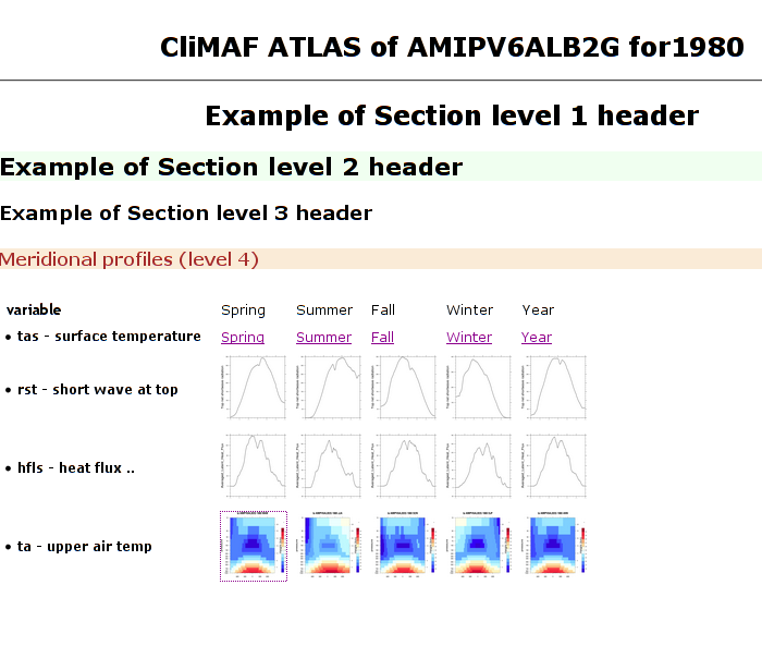

climaf.html.header(title, style_file=None)

Returns text for an html document header, with provided title. If a style filename is not provided, a default style sheet will apply

climaf.html.trailer()

Returns the text for closing an html document

climaf.html.section(title, level=1, key='None')

Returns text for a section header in an html document with given title. Style depends on level value. Arg key is not yet used

climaf.html.open_table(title='', columns=[], spacing=5)

Returns header text for an html table. title will go as title for first column. columns should be a list of column titles

climaf.html.close_table()

Returns text for closing an html table

climaf.html.open_line(title='')

climaf.html.close_line()

climaf.html.line(list_of_pairs, title='', thumbnail=None, hover=True, dirname=None, altdir=None)

Create an html line with labels and links from first args list_of_pairs (and when this is not a pair, only put the label). Put a line title if provided. Replace labels with thumbnail figures if arg thumbnail is set to a size (in pixels) and display figures when you mouse over it if arg hover is set to True or to a size (in pixels); in that case, dic can also be a list of filenames. If ‘dirname’ is not None, creates hardlinks to the filenames, in directory dirname, and named as ‘climaf_atlas’([0-9]+).ext (where ‘ext’ is ‘png’, ‘pdf’ or ‘eps’). This allows to generate a portable atlas in dirname

climaf.html.link(label, filename, thumbnail=None, hover=True)

Creates the provided label, with a link to the provided image filename (if not None) and possibly showing a thumbnail for the image (with the provided thumbnail size) and possibly displaying this image when mouse is over it (with the provided hover size).

• ‘thumbnail’ can be an integer or a string with width or height (in these cases, width=height), or a string with width and height separated by character ‘x’ or ‘*’. The size is in pixels; default : None (no thumbnail)
• ‘hover’ can be a logical, or a string with width or height (in this case, width=height), or a string with width and height separated by character ‘x’ or ‘*’. The size is in pixels; default is True, which tanslates according to value of thumbnail :
  • if thumbnail is not None, hover width and height are respectively set as 3 times that of thumbnail width and height
  • if thumbnail is None, size is ‘200*200’

climaf.html.link_on_its_own_line(label, filename, thumbnail=None, hover=True)

Does the same as link() ,but for a link which is sole on its own line

climaf.html.cell(label, filename=None, thumbnail=None, hover=True, dirname=None, altdir=None)

Create a table cell with the provided label, which bears a link to the provided filename and possibly shows a thumbnail for the link with the provided thumbnail size (in pixels) and possibly display it when you mouse over it (with the provided hover size in pixels).

If ‘dirname’ is not None, creates a hard link in directory dirname to file filename. This allow to generate a portable atlas in this directory. Hard links are named after pattern climaf_atlas<digit>.<extension>

‘dirname’ can be a relative or absolute path, as long as filename and dirname paths are coherent

If ‘altdir’ is not None (and ‘dirname is None), the HREF links images in index have the prefix of their absolute path changed from $CLIMAF_CACHE to ‘altdir’ (use case : when the Http server only knows another filesystem). Example:

• CLIMAF_CACHE=/prodigfs/ipslfs/dods/fabric/coding_sprint_NEMO/stephane
• URL https://vesg.ipsl.upmc.fr /thredds/fileServer/IPSLFS/fabric/coding_sprint_NEMO/stephane/ .../fig.png

climaf.html.fline(func, farg, sargs, title=None, common_args=[], other_args=[], thumbnail=None, hover=True, dirname=None, **kwargs)

Create the html text for a line of table cells, by iterating calling a function, once per column, with at least two arguments. Cells have a label and possibly a link

• ‘func’ is a python function which computes and labels and/or figures;
• ‘farg’ is any object, used a 1st arg for ‘func’;
• ‘sargs’ is a list or a dict, used for providing the 2nd arg to each call to ‘func’.
• ‘title’ is a line title (for first column); if missing, ‘farg’ is used
• see further below fo remaining arguments

So, there will be one column/cell per item in ‘sargs’; each cell shows a label which can be an active link. Both the label value and the link value can be the result of calling ‘func’ arg with the pair of arguments (‘farg’ and the running element of ‘sargs’); the function can return a single value (either a label or a figure filename) or both

Use cases :

• a line showing just numeric values; we assume that function average(var,mask) returns such a numeric value, which is a gloabl average of a variable over a mask:

  >>> rep=fline(average, 'tas',        ...   [ 'global', 'sea', 'land', 'tropics'], 'tas averages')
  

• a line showing the same average values, but each value is a link to e.g. a figure of the time series of global average values : same call, but just let function ‘average’ compute the average and the figure, and return a couple : average, figure filename

• a line showing pre-defined labels, which here are shortcuts for mask names, and which carry links to same figures as above : let function ‘average’ only return the figure filename, and call :

  >>> rep=fline(average, 'tas',
  ...  {'global':'GLB','sea':'SEA','land':'LND'}, 'tas averages')
  

Advanced arguments :

• common_args : a list of additionnal arguments to pass to ‘func’, whatever the value of its second argument
• other_args : a dictionnary of lists of additionnal arguments to pass to ‘func’; only the entry which key equals running value of second argument is passed to ‘func’ (after common_args)
• thumbnail : if ‘func’ returns a filename, generate a thumbnail image of that size (in pixels)
• hover : if ‘func’ returns a filename, display image of that size (in pixels) when you mouse over it. If hover is True:
  • hover width and height are respectively set as 3 times that of thumbnail width and height if thumbnail is not None
  • hover is set to ‘200*200’ if thumbnail is None
• dirname : if ‘func’ returns a filename, creates a directory (if doesn’t exist) wich contains filename as a hard link to the target dirname/’climaf_atlas’([0-9]+).ext (‘ext’ is ‘png’, ‘pdf’ or ‘eps’)

climaf.html.flines(func, fargs, sargs, common_args=[], other_fargs=[], other_sargs=[], thumbnail=None, hover=True, dirname=None, **kwargs)

See doc for fline() first

Creates a table by iterating calling fline over ‘fargs’ (which can be a list or a dict) with :

• ‘farg’ being the running element (or key) of ‘fargs’
• ‘title’ being the corresponding ‘fargs’ value (or ‘farg’ if not a dict)
• ‘common_args’ being forwarded to fline()
• ‘other_args’ being the merge of other_fargs[farg] and other_sargs

It forwards remaining keyword arguments (kwargs) to fline()

Example : assuming that function avg returns the filename for a figure showing the average value of a variable over a mask, create a table of links for average values of two variables over two masks, with thumbnail of images and displaying images when you mouse over it with ‘hover’ argument:

>>> t=table_lines(avg,['tas','tos'],['land','sea'],thumbnail=40,hover='60x80')

climaf.html.vspace(nb=1)